Introduction
This homework mainly focuses on the calculation of the structural stability and phase diagrams of diamond and β-Sn structured silicon, and vibrational properties of silicon and $\rm PbTiO_3$. In exercise 1, the lattice constants and cohesive energies from the given equation. It is also computationally verified that the diamond structure is more stable than β-Sn silicon by 0.2501 eV/atom. Comparison with experimental data shows that ... In exercise 2, the relation of total enthalpy to the volume of silicon atoms is visualized and the equilibrium structures are identified at different pressures. It is verified that 9.6 GPa is the critical pressure, under which the two phases of silicon are equally stable. In exercise 3, the phonon dispersion curve considering different volume changes is plotted. Then the bulk modulus of silicon is computed from the elastic constants. The elastic constants of $\rm PbTiO_3$ are calculated by applying different strains. The thermal coefficients are thence obtained from the elastic constants.
import numpy as np
import matplotlib.pyplot as plt
from matplotlib import rcParamsDefault
from datascience import Table
import scipy
%matplotlib inline
Exercise 1: Structural Stability of Different Phases at Zero Pressure
Exercise 1A
Using the data in Table 1, determine the lattice parameters and the cohesive energies of silicon in the two phases at equilibrium (this is most easily accomplished by plotting the data and fitting the points to some low-order polynomial to determine the minimum), and verify that at ambient conditions the diamond structure is more stable than the β-Sn structure by 0.25 eV/atom.
The data are plotted in MATLAB and fitted in the curve fitting toolbox with a 4th order polynomial function shown below, where the fitting parameters are listed as below. The lowest point is obtained through finding the min point of the fitted function. The ambient condition structure energy difference are obtained through calculating the difference of the two fitted lowest points.
![]()
![]()
To obtain an accurate representation of the data fit, fourth order polynomial fitting functions are employed where the details are listed below:
- Model for fitting the silicon $E_c$: $E_c(a) = p_1 a^4 + p_2 a^3 + p_3 a^2 + p_4a + p_5$
Coefficients for diamond silicon structure (with 95% confidence bounds): $$p_1 = 0.5904\quad (0.5494, 0.6314)$$ $$p_2 = -13.71\quad (-14.53, -12.89)$$ $$p_3 = 120.5\quad (114.4, 126.7)$$ $$p_4 = -474.1\quad (-494.3, -453.9)$$ $$p_5 = 697.3\quad (672.5, 722.1)$$ SSE: 0.001007; R-square: 1; Adjusted R-square: 1; RMSE: 0.007934
Coefficients for β-Sn structure (with 95% confidence bounds): $$p_1 = 0.474\quad (0.4461, 0.5018)$$ $$p_2 = -10.63\quad (-11.19, -10.07)$$ $$p_3 = 89.6\quad (85.44, 93.76)$$ $$p_4 = -334.9\quad (-348.6, -321.2)$$ $$p_5 = 462.1\quad (445.2, 478.9)$$ SSE: 0.0004643; R-square: 0.9999; Adjusted R-square: 0.9999; RMSE: 0.005387
Given the fitted functions the cohesive energies can be obtained through calculating the lowest point of the fitting function: for diamond silicon, the minimum value (cohesive energy) is -5.309 eV/atom, and for β-Sn, the minimum value (cohesive energy) is -5.0508 eV/atom. The lattice constants for diamond and β-Sn silicon are 5.42 Å and 4.77 Å, respectively.
As for verfying the stability of the two structures under ambient conditions, the difference between the lowest point of the two fitting functions can then be obtained: $\Delta E = |5.0508 - 5.3009| = 0.2501 \rm eV$.
According to the work by Hu et al., the lattice constant for diamond silicon (at 11.3 GPa) is $5.268 \pm 0.010Å$ and for β-Sn is $4.69\pm0.006Å$. My fitted results indicate the lattice constants for the two structured silicon are 5.42 Å and 4.77 Å, respectively. If taking the reference as a benchmark, the relative errors of the fitted parameters are 2.89% and 1.71%, respectively.
Exercise 2: Structural Stability and Phase Diagrams Under Pressure
Exercise 2A
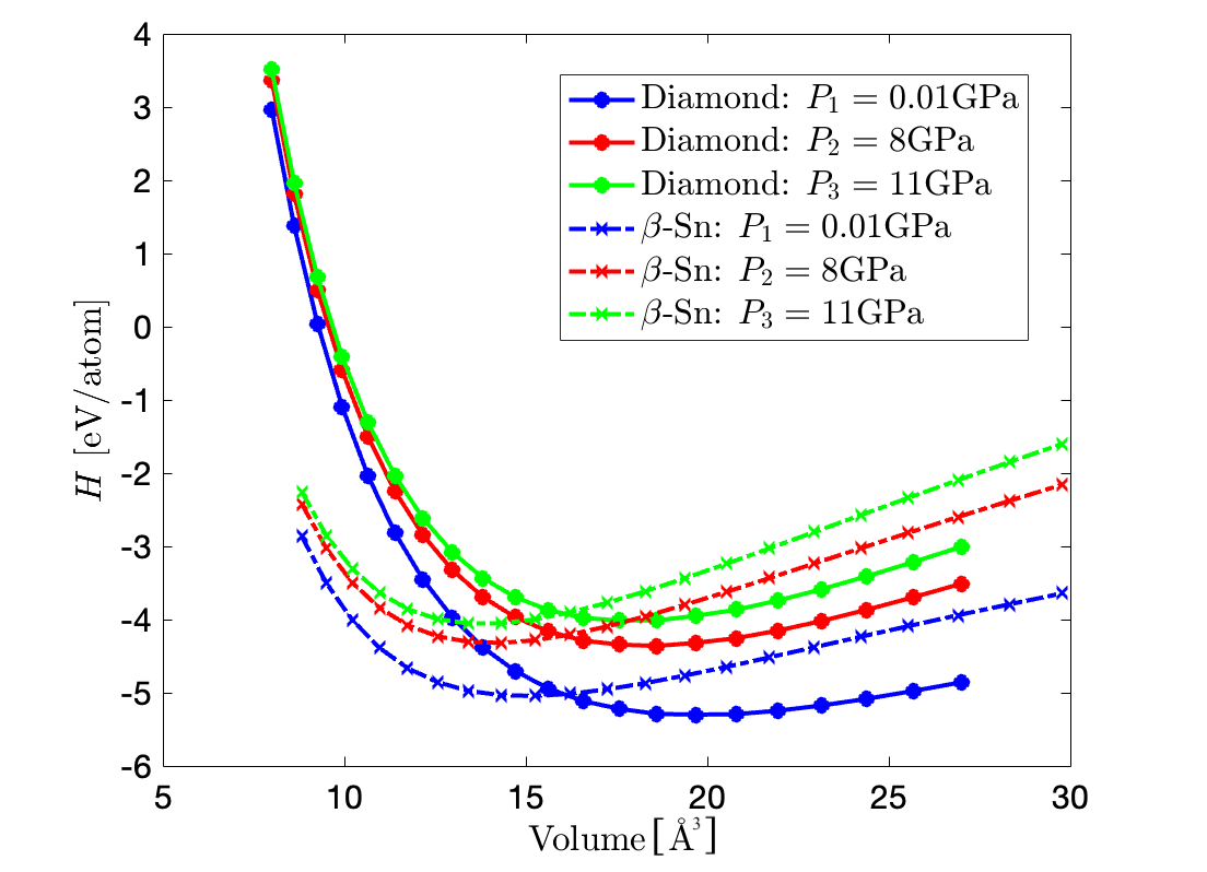
Using the data in Table 1 plot the enthalpy of silicon (in eV) as a function of the volume per atom (in $Å^3$), both for the diamond structure and the β-Sn structure, for the pressures $P_1$ = 0.01 GPa, $P_2$ = 8 GPa, and $P_3$ = 11 GPa.
According to the given equation $H = U + PV$. Considering the given fixed ratio of $\frac{c}{a} = 0.5516$. According to Equation (1), we know that $U = (E_c + E_{\rm Si} )M$. Since the unit for energies is $\rm eV/atom$, hence $M = 1$. Regarding the volume computation, the volumes are computed from the equation $V = (\mathbf{a}_1 \times \mathbf{a}_2) \cdot \mathbf{a}_3$ (Prof. Sun's website), where the three main primitive vectors are obtained based from Prof. Leitner's website (link 1 & link 2).
Exercise 2B
Identify the equilibrium structure at each one of the three pressures, $P_1$, $P_2$ and $P_3$.
We identify the lowest point of the fitting function for the three different structured silicon considering different pressures with the same procedure as above, and listed as below. The corresponding lattice constants are hence presented.
diamond_2b = [-5.314, -4.348, -4.004]
volume_diamond_2b = [20.18, 18.55, 18.13]
beta_2b = [-5.054, -4.335, -4.075]
volume_beta_2b = [14.81, 13.92, 13.78]
pressure = ['P1 = 0.01','P2 = 8', 'P3 = 11']
tab_2b = Table().with_columns(['Pressure Values [GPa]', pressure, 'Diamond Energy [eV]', diamond_2b, 'β-Sn Energy [eV]', beta_2b, \
                               'Diamond Volume [Å3]', volume_diamond_2b, 'β-Sn Volume [Å3]', volume_beta_2b])
tab_2b
Exercise 2C
Verify that the critical pressure at which the two phases are equally stable is 9.6 GPa, and compare this calculated LDA value with the experimental data from Hu, et al.
To verify the given critical pressure, the enthalpy of different silicon structures regarding to the volume are plotted shown below. The pressure comparisons are presented zoomed in the range of $[-4.3, 4]$ eV/atom for presenting the differences of the fitted lowest points. It is verified at 9.6 GPa the two lowest energy are at the same level.
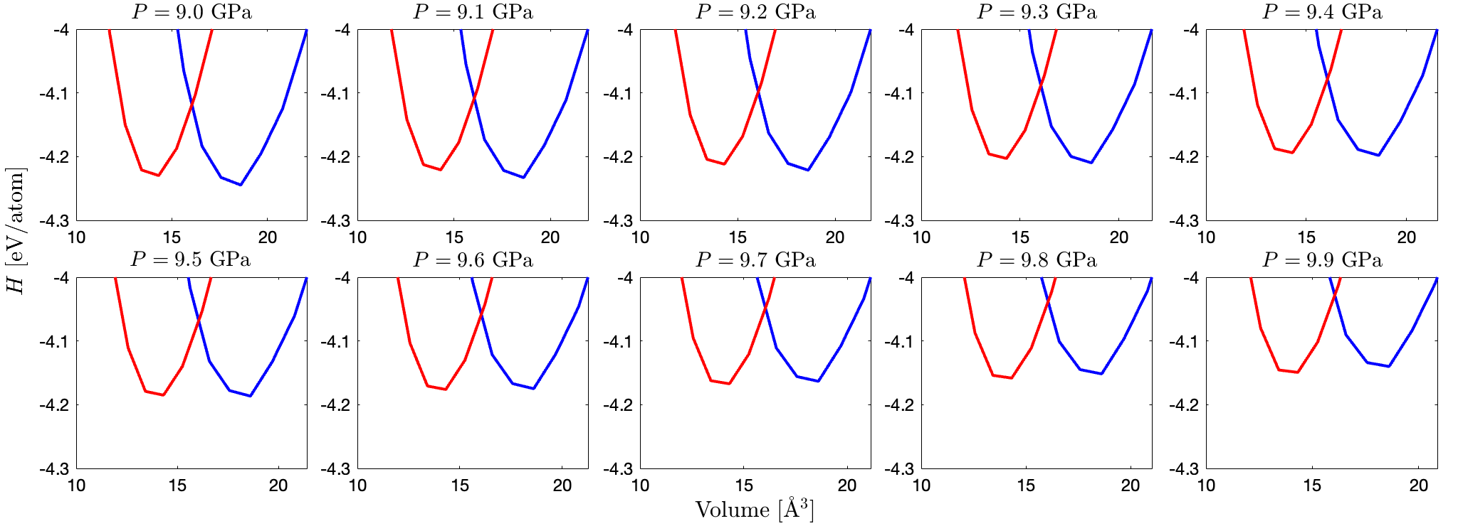
For 9.6 GPa, the lowest point of the curve are found through going through the curve from the 4th order polynomial fit (same as in exercise 1). From the gievn figure it can be observed that for diamond silicon the lowest enthalpy is -4.19 eV/atom and for β-Sn silicon is -4.16 eV/atom. Both the two lowest values can be approximated as -4.2 eV/atom, as visualized in the gray dashed line in the figure. Hence the given critical value is verified.
![]()
In the work of Hu et al., the transition pressure from the β-Sn (Phase II) to diamond (Phase III) ranges from 8.5 to 10.8 GPa. The calculated LDA value (9.6 GPa) lies in this general range.
Exercise 3: Vibrational Properties of Solids
Exercise 3A
Calculate the phonon dispersion curve of silicon on a $4\times4\times4$ q-point grid for the equilibrium volume, a volume 5% larger than equilibrium and a volume 5% smaller. Present all three curves on the same plot. Notice which phonon modes change their frequencies as the volume changes.
From my HW2, the calculated equilibrium lattice constant of aluminum is 10.1941Å. When the total volume of the primitive cell are deformed $\pm 5\%$), the corresponding lattice constants are 10.0213 and 10.3614 Å, respectively. Recalling HW2 we also know that optimal cutoff energy is 30 Ry, respectively. Applying these parameters and compute the phonon dispersion we hence generate the following figure, where the blue line denotes the undeformed silicon and the black and red lines denote the silicon are deformed +5% and -5%.
![]()
Exercise 3B
Calculate the bulk modulus for silicon based on calculations performed for previous homework assignments.
According to the given equation: $$B = \frac{1}{3} (C_{11} + 2C_{12})$$
Based on the results from HW2, the values of the two elastic constants: $C_{11} = 163.78\rm GPa$ and $C_{12} =65.22\rm GPa$. The bulk modulus of silicon is $B = 98.0733\rm GPa$. If taking the work by George [2] as a reference, the bulk modulus of silicon is 97.84GPa, my computed results has a relative error of 0.24%.
Exercise 3C
Calculate the relevant elastic constants for $\rm PbTiO_3$ and invert the matrix to find the elements of $\bf S$ required to evaluate $α_a$ and $α_c$. You will need to fully relax the lattice constants and atomic coordinates first. Since $\rm PbTiO_3$ is not cubic, you will also need to relax the atomic coordinates for each strain value.
The energy cutoff and lattice constants of $\rm PbTiO_3$ ae first converged using the same methods as in HW1, where the convergence criteria is met when the energy difference is less than 10 meV/Å, same as in HW1:
cutoff_PTO = np.array([20,30,40,50,60,70,80,90,100,110,120,130,140,150])
ener_PTO_cutoff = np.array([-379.78776305,-380.54586804,-380.57263600,-380.57404325,-380.57535043,-380.57580974,-380.57642195,-380.57706326,\
                            -380.57744076,-380.57754407,-380.57763330,-380.57783156,-380.57802507,-380.57811993])
ener_PTO_diff = np.abs([ener_PTO_cutoff[1]-ener_PTO_cutoff[0],ener_PTO_cutoff[2]-ener_PTO_cutoff[1],ener_PTO_cutoff[3]-ener_PTO_cutoff[2],\
                        ener_PTO_cutoff[4]-ener_PTO_cutoff[3],ener_PTO_cutoff[5]-ener_PTO_cutoff[4],ener_PTO_cutoff[6]-ener_PTO_cutoff[5],\
                        ener_PTO_cutoff[7]-ener_PTO_cutoff[6],ener_PTO_cutoff[8]-ener_PTO_cutoff[7],ener_PTO_cutoff[9]-ener_PTO_cutoff[8],\
                        ener_PTO_cutoff[10]-ener_PTO_cutoff[9],ener_PTO_cutoff[11]-ener_PTO_cutoff[10],ener_PTO_cutoff[12]-ener_PTO_cutoff[11],\
                        ener_PTO_cutoff[13]-ener_PTO_cutoff[12]])
fig, axs = plt.subplots(1, 2, figsize = (15, 5))
axs[0].plot(cutoff_PTO[1:14], ener_PTO_diff, '-.')
axs[0].plot(cutoff_PTO[1:14], ener_PTO_diff, 'ro')
axs[0].plot([30, 150], [3.8894e-04, 3.8894e-04], '-')
axs[0].text(30, 0.0005, '$\delta_{Force} = 10$ [meV/$\AA$]')
axs[0].set_xlabel('Energy cutoff [Ry]')
axs[0].set_ylabel('|$\mathcal{E}_{Energy}$| [Ry/bohr]')
axs[0].set_yscale('log')
axs[1].plot(cutoff_PTO, ener_PTO_cutoff, '-.')
axs[1].plot(cutoff_PTO, ener_PTO_cutoff, 'ro')
axs[1].set_xlabel('Energy cutoff [Ry]')
axs[1].set_ylabel('Energy [Ry/bohr]')
kpoint_PTO = np.array([6,7,8,9,10])
ener_PTO_kpoint = np.array([-380.57744076,-380.57769125,-380.57770635,-380.57771768,-380.57768939])
ener_k_diff = np.abs([ener_PTO_kpoint[1]-ener_PTO_kpoint[0],ener_PTO_kpoint[2]-ener_PTO_kpoint[1],\
                      ener_PTO_kpoint[3]-ener_PTO_kpoint[2],ener_PTO_kpoint[4]-ener_PTO_kpoint[3]])
fig, axs = plt.subplots(1, 2, figsize = (15, 5))
axs[0].plot(kpoint_PTO[1:5], ener_k_diff, '-.')
axs[0].plot(kpoint_PTO[1:5], ener_k_diff, 'ro')
axs[0].plot([7, 10], [3.8894e-04, 3.8894e-04], '-')
axs[0].text(8.5, 0.00028, '$\delta_{Force} = 10$ [meV/$\AA$]')
axs[0].set_xlabel('k point')
axs[0].set_ylabel('|$\mathcal{E}_{Energy}$| [Ry/bohr]')
axs[0].set_yscale('log')
axs[1].plot(kpoint_PTO, ener_PTO_kpoint, '-.')
axs[1].plot(kpoint_PTO, ener_PTO_kpoint, 'ro')
axs[1].set_xlabel('k point')
axs[1].set_ylabel('Energy [Ry/bohr]')
From the above figures it can be deduced that the converged energy cutoff and k points for $\rm PbTiO_3$ are 100 Ry and [7, 7, 5], respectively.
we first compute the converged lattice constant using method 'vc-relax', the converged lattice constants matrix ($\tt CELL\_PARAMETERS$)
$\tt CELL\_PARAMETERS\ (angstrom)$
$\tt 3.855813126\quad 0.000000000\quad 0.000000000\\0.000000000\quad 3.855813126\quad 0.000000000\\0.000000000\quad 0.000000000\quad 4.051423221$
$\tt ATOMIC\_POSITIONS\ (crystal)$
$\tt Pb\quad 0.0000000000\quad 0.0000000000\quad 1.0051904083 \\ Ti\quad 0.5000000000\quad 0.5000000000\quad 0.5395123895 \\ O\quad\ 0.5000000000\quad 0.5000000000\quad 0.0994787311\\ O\quad\ 0.5000000000\quad 0.0000000000\quad 0.6115513795\\ O\quad\ 0.0000000000\quad 0.5000000000\quad 0.6115513795$
Following the same procedure as in HW2, we apply the 'relax' calculation methods. For the cell parameters $\mathcal{C}$, considering different different strains $\eta = [-0.006, -0.004, -0.002, 0, 0.002, 0.004, 0.006]$, $\mathcal{C}$ are computed as follows:
where $\mathbb{C}$ denotes the undeformed primitive cell box cell parameters and $\mathbf T$ are given in the instructions. We also generate a MATLAB code to obtain the cell parameters for deforming the primitive cell. Note that the undeformed volume $V_0$ of the primitive cell is 406.4721 $\rm bohr^3$.
Substitute the above contents into the in script and obtain the elastic constants from the given instructions: taking different strains, then the second-order parameters can be fitted as follows:
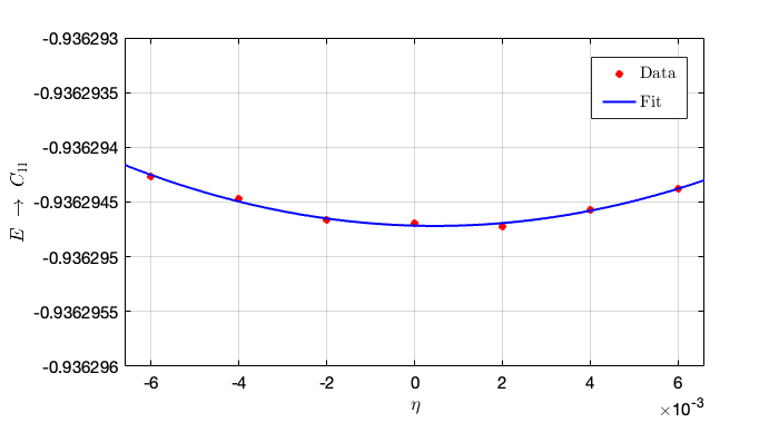
- From this figure we can conclude that the second-order fit is $C_{11} = 14710.5\times 0.01311 = 192.8547 \rm GPa$.
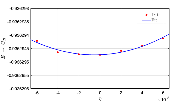
- From this figure we can conclude that the second-order fit is $C_{33} = 14710.5\times 0.0154 = 226.5417 \rm GPa$.
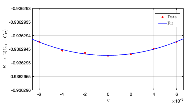
- From this figure we can conclude that the second-order fit is $2(C_{11} - C_{12}) = 14710.5\times 0.01382 = 203.2991 \rm GPa$. Hence, we can compute $C_{12} = 192.8547 - 101.6496 = 91.2051 \rm GPa$.
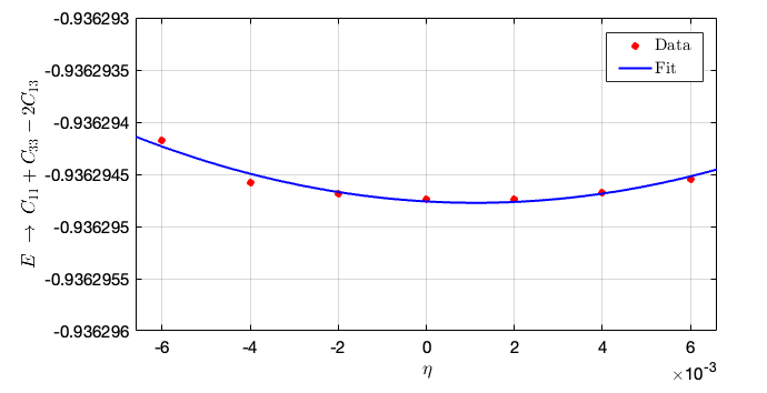
- From this figure we can conclude that the second-order fit is $C_{11} + C_{33} - 2C_{13} = 14710.5\times 0.01064 = 156.5197 \rm GPa$. Hence, we can compute $C_{13} = \frac{192.8547+226.5417-156.5197}{2} = 131.4384 \rm GPa$.
We can thence write out the matrix for elastic constants: $$ \mathbf{C} = \begin{bmatrix} 192.8547 & 91.2051 & 131.4384\\ 91.2051 & 192.8547 & 131.4384\\ 131.4384 & 131.4384 & 226.5417 \end{bmatrix} $$
Writing in the SI unit (Pascal), the matrix writes:
$$ \mathbf{C} = \begin{bmatrix} 192.8547\times 10^9 & 91.2051\times 10^9 & 131.4384\times 10^9\\ 91.2051\times 10^9 & 192.8547\times 10^9 & 131.4384\times 10^9\\ 131.4384\times 10^9 & 131.4384\times 10^9 & 226.5417\times 10^9 \end{bmatrix} $$By inverting the matrix we can obtain $\bf S$ (in reverse of GPa): $$ \mathbf{S} = \begin{bmatrix} 0.0087 & -0.0011 & -0.0044\\ -0.0011 & 0.0087 & -0.0044\\ -0.0044 & -0.0044& 0.0095\\ \end{bmatrix} $$
Therefore, the elements of $\bf S$ for evaluating the thermal coefficients can be obtained: $S_{11} = 0.0087,\ S_{33} = 0.0095,\ S_{12} = -0.0011,\ S_{13} = -0.0044$.
Exercise 3D
While E. Coyote of Acme Labs measured the bulk Grüneisen parameters for silicon and $\rm PbTiO_3$. For Si, he measured a value of $γ_{bulk} = 2$ and for $\rm PbTiO_3$, he obtained the results $γ_{bulk}^c = 0.4$ and $γ_{bulk}^a = 1.7$. Using these values, and your calculated results for the bulk modulus of Si and the compliance matrix elements for $\rm PbTiO_3$, evaluate $α_v$ for silicon and $α_a$ and $α_c$ for $\rm PbTiO_3$. A negative value of $α$ means that the material undergoes negative thermal expansion. Do either Si or $\rm PbTiO_3$ exhibit negative thermal expansion? Note that for $\rm PbTiO_3$ you should evaluate $\alpha_v = 2α_a +\alpha_c$. Thermal expansion coefficients have units of inverse temperature. Since we are only estimating the coefficients (the expressions above are missing some unimportant – for us – constants), they will have units of inverse pressure, since Grüneisen parameters are dimensionless. Is negative thermal expansion observed experimentally for either Si or $\rm PbTiO_3$?
For $\rm PbTiO_3$, taking the equations from the instructions, we write:
$$\alpha_a \sim \left[ (S_{11} + S_{12})\gamma_{\rm bulk}^a + S_{13} \gamma_{\rm bulk}^c \right] $$and $$\alpha_c \sim \left[ 2 S_{13} \gamma_{\rm bulk}^a + S_{33} \gamma_{\rm bulk}^c \right] $$
From Exercise 2, we substitute the obtained $S$ values into the equations and compute the corresponding thermal expansion coefficients:
$$ \alpha_a \sim (0.0087 - 0.0011) \times 0.4 - 0.0044 \times 1.7 = -0.0044\\ \alpha_c \sim 2 \times (-0.0044) \times 0.4 + 0.0095 \times 1.7 = 0.0126 $$we then obtain $\alpha_v = 2\alpha_a + \alpha_c = 0.0038\times \rm \ GPa^{-1}$.
It can be deduced that $\rm PbTiO_3$ does not possess a negative thermal coefficient.
For silicon, the thermal coefficient writes: $\alpha = \frac{\gamma_{bulk}}{B} = \frac{2}{98.0733}\times 10^{-9} = 0.0204\rm \ GPa^{-1}$.
It can be deduced that silicon does not possess a negative thermal coefficient.
Summary
In this homework, we were assigned to compute the structural stability of different phases of silicon in which I learned how to determine the phase transition of solid materials. Also, it is better understood how to employ the powerful tool of curve fitting to determine cohesive energies, lattice constants, etc. The thermal and vibrational properties of different solid materials (silicon & $\rm PbTiO_3$) were computed from Quantum ESPRESSO.
During the homework process I find the following point important and worth noticing:
Determine the order of fitting functions for cohesive energies and lattice parameters is a critical step, yet highly empirical. If the order is too low yet there are abundant data from the first-principle computation, then the curve fitting may be inaccurate, leading to many data points lying out of the fitted curve. If the order is too high yet there are very few computed data, the curved may be overfitted, leading to a bad representation of materials properties. Hence, more practice and literature references are significant regarding modeling from curve fitting in solid materials computation.
First principle computation of elastic constants tends to be highly sensitive. When applying different strains, the corresponding energies are sensitive to lattice constants, k points, etc.
First principle computation of thermal and vibrational properties tends to be computationally expensive. As already mentioned by Prof. Benedek, the calculation of phonon dispersion is very slow. I proposed the following explanation: When probing the phonon to compute the vibrational properties, the silicon structure is reconstructed where the optimization of the structure took a long computation time.
Also, I encountered the following difficulties during the process, and solved them correspondingly:
When applying different strains for computing the phonon dispersion curve, the figure did not look quite correct at the beginning. As I double-checked it, the following two reasons caused it: (1) I didn't type the correct lattice constants to apply the strains, as the $\pm 5\%$ corresponds to total volume change rather than the lattice constants change. (2) I tried to generate the figure by copy-paste the data by directly editing the
.psfiles, yet the results don't look quite correct.I got confused on how to correctly apply the strains initially. After I asked Sabrina and discussed it with Mads I realize my original idea (by setting $\tt celldm(1)$ and $\tt celldm(3)$ to the computed $a$ and $c$) was not easy to implement. I then did the matrix multiplication as I wrote and then apply the strains to the $\rm PbTiO_3$ primitive cells.
References
[1] Hu, J. Z., Merkle, L. D., Menoni, C. S. and Spain, I. L. “Crystal data for high-pressure phases of silicon” Physical Review B 34 4679 (1986). 10.1103/PhysRevB.34.4679
[2] A. George, “Elastic constants and moduli of diamond cubic Si,” in EMIS. Datareviews, vol. 20, Properties of Crystalline Silicon, R. Hull, Ed. London, U.K.: INSPEC, 1997, p. 98. [PDF].